DAQ/Advanced/Temperature Measurement using RTD through Scilab and PCI 1711/English
Temperature Measurement using RTD through Scilab and Data Acquisition Hardware, PCI 1711
This tutorial explains the step by step procedure to measure temperature using RTD through Scilab and Data Acquisition Hardware in a Linux operating system. The hardware used is Advantech PCI 1711 multifucntion DAQ card. Note that you cannot use Advantech PCI card in your laptop. So you need a PC with atleast one PCI slot on the motherboard. Hope you have installed the required packages for using this hardware for Data acquisition. To install these, refer to our tutorial on the same in the DAQ main page.
You need the following hardware:
   1. Advantech PCI 1711 with cable and ADAM module 3968 SCSI 68P Terminal Board.
   2. Multi output dual power supply (+12 ,-12 V and 3.3V).
   3. Signal conditioning circuit, Here is the circuit.
Hope you have inserted the DAQ card in the PCI slot. Do not forget to load the module corresponding to PCI 1711 DAQ card, which is done by typing the following command in the Linux terminal:
$ modprobe adv_pci1710
To check the COMEDI device name associated with your DAQ card, and if the card has been identified by the OS , do the following:
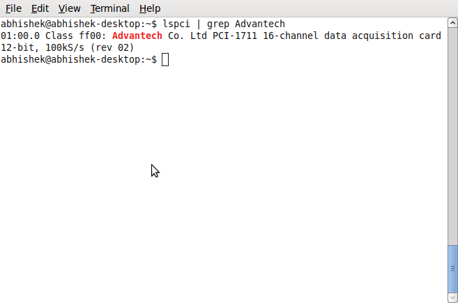
$ lspci | grep Advantech, This gives:
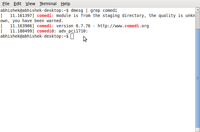
$ dmesg | grep comedi , This gives:
Here the PCI 1711 is assigned to comedi0. This is the device name.
If you do not get these messages, then re-check your software installation.
Note that the setup could also be used for Measurement Computing DAQ card PCI-DAS1002. I will call it MCC card from now on. If you are using MCC card do,
$ modprobe cb_pcidas
For MCC card, the commands:
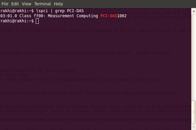
$ lspci | grep PCI-DAS1002
gives:
and
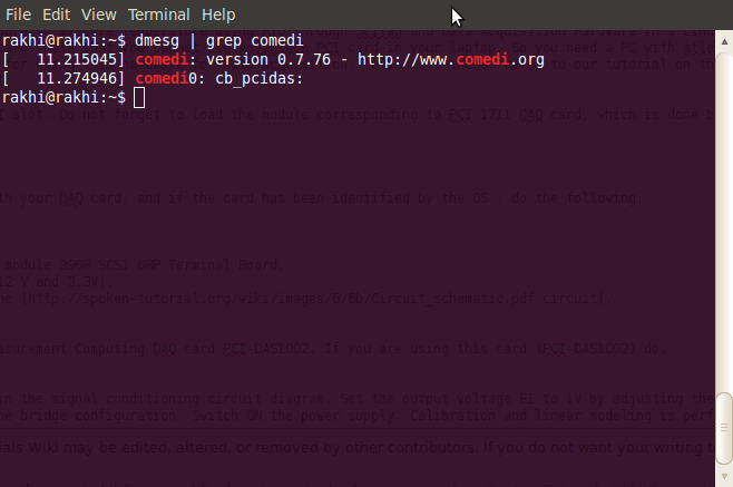
$ dmesg | grep comedi
gives:
Hope you have connected the circuit as given in the signal conditioning circuit diagram. Set the output voltage E1 to 1V by adjusting the 1k pot R1. This ensures that a constant current of 1mA excites the wheat-stone bridge configuration. Switch ON the power supply. Calibration and linear modeling is performed as given below:
The linear model is
<math>t = a*Vout + b</math>
For E1, Vo, Vout, R1, R9 etc, refer the circuit diagram given above.
Dip the RTD in ice at 0 degree Celsius. At 0 degree, measure the voltage Vo. Adjust the pot R9 such that Vo is zero. It may not become zero. There will be a slight error or offset. Measure the corresponding amplified output Vout. Substitue in the above equation.
<math>0 = a*Vout + b</math>..................(1)
Take another reference temperature,say 100 degree Celsius. Measure Vout.
<math>100 = a*Vout + b</math>.................(2)
Solve the equations (1) and (2) to get values of a and b.
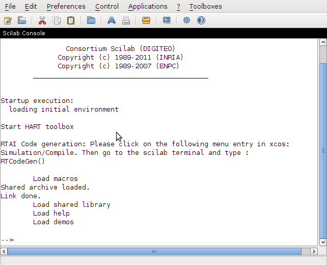
Now let us begin the experiment. Open the Scilab console window. If the HART toolbox is properly installed you can see hart_0.4.3 under Toolboxes. Click on hart_0.4.3. You will get the following message on the Scilab console window.
This indicates that the HART toolbox is loaded properly. Otherwise, you will get error messages. Change the working directory to the one where your code is saved. For me, it is in
/home/abhishek/Desktop/daq/DAQ_xcos_files.
You require the following files:
      1. find_temp.sci Download it from here
      2. rtd_affich_linear.xcos Download it from here (To save the xcos file, right click on the link
         and choose 'save link as')
Switch on the power supply. Substitute the values of a and b that you have calculated above in the find_temp.sci file. Execute the find_temp.sci file. This is a very simple code which linearly models the RTD output voltage and temperature. The code is reproduced below for your convenience.
       mode(-1);
       function [t] = find_temp(vo)

       //vo is the amplified output of the wheatstone bridge
       // t is temperature output.
       // the linear model is t = 34.742*vo + 0.21109
      //You may have to use your own calibrated values for a and b
      //t = av+b;
      a = 34.742;
      b = 0.21109;
      t = a*vo + b;
      endfunction
(To know more about Scilab and Xcos, refer to the spoken tutorial on Scilab).
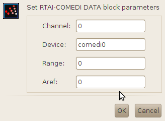
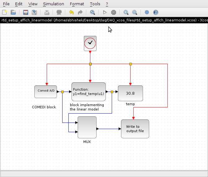
Open Xcos. Open rtd_affich_linear.xcos. Double click on the COMEDI A/D block. Adjust the parameters as shown below:
Channel is the analog channel of the DAQ to which the input is connected. Device is the COMEDI device name. We have the device name as comedi0. This is already explained. For, Range and Aref you can give a safe value of 0. You may want to refer the Xcos help for the COMEDI A/D block to know more.
Click on the play button in the Xcos window. You can see that you start getting the temperature on the block named temp as given below.
The blocks are added to the Xcos diagram using Palette Browser. It gets opened up when you open Xcos or you can get it in the Xcos diagram from View-->Palette Browser. 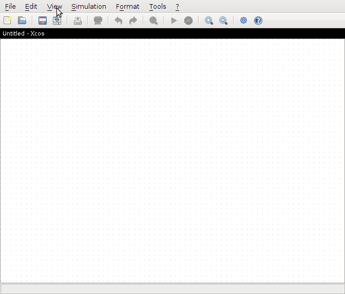
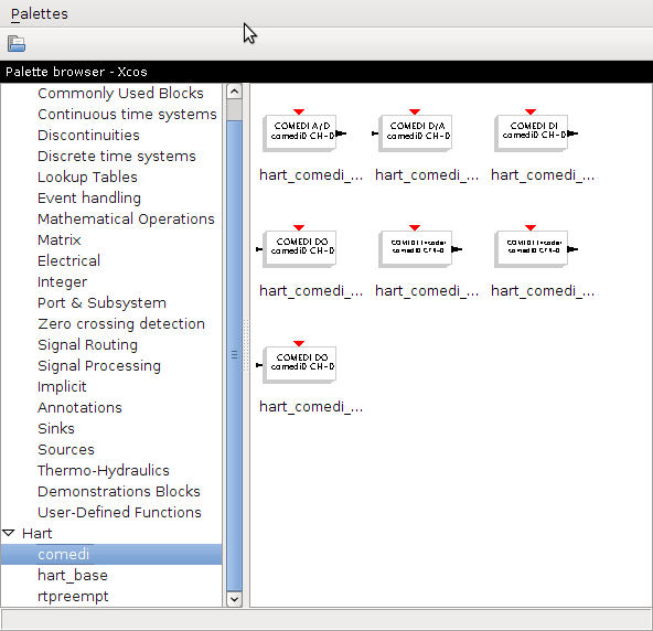
COMEDI blocks are available in the hart palette.Click on Hart palette. Click on comedi. The blocks are as shown below:
This brings us to the end of this tutorial. This is Rakhi for DAQ project. Thanks. Goodbye.
